本文共 3135 字，大约阅读时间需要 10 分钟。

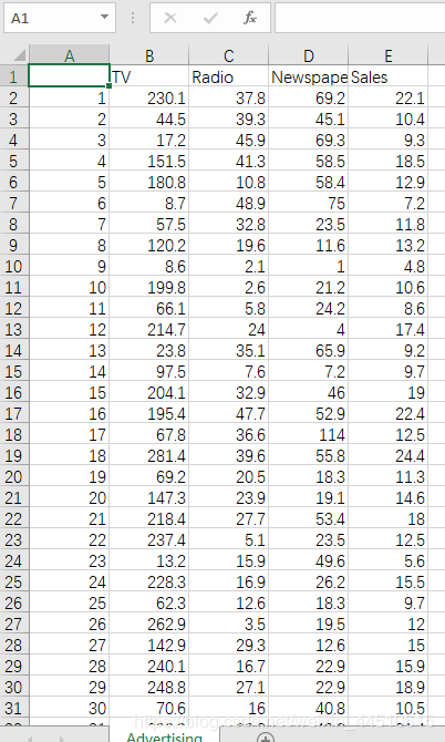
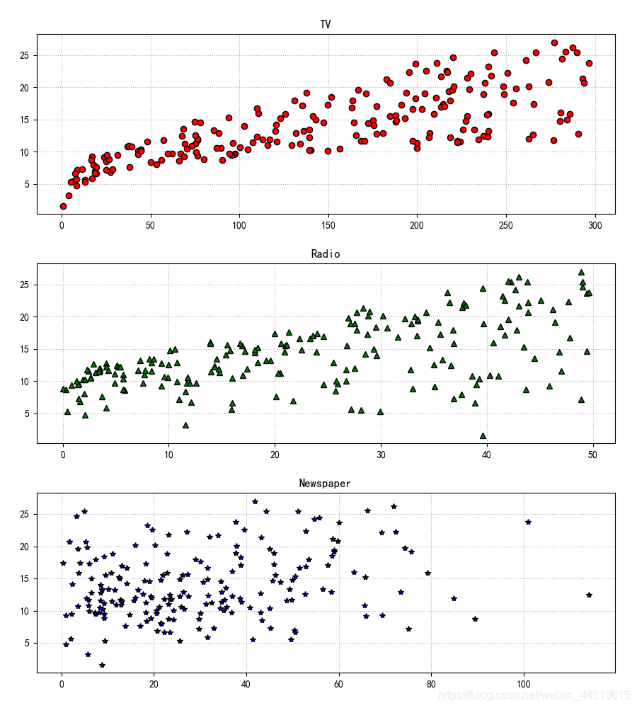
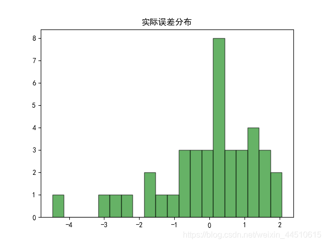
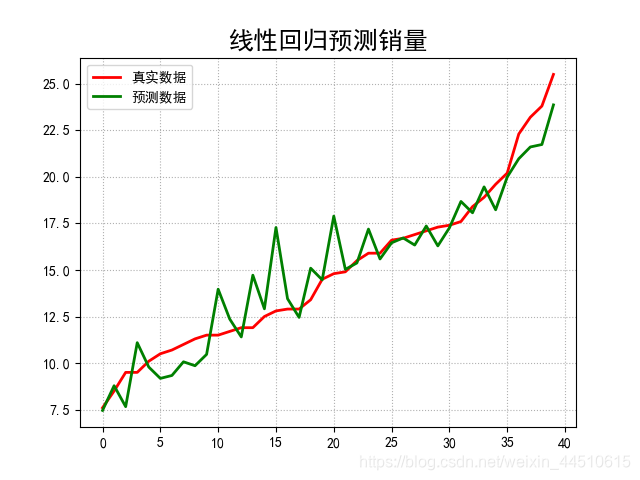
#!/usr/bin/python# -*- coding:utf-8 -*-import csvimport numpy as npimport matplotlib as mplimport matplotlib.pyplot as pltimport pandas as pdfrom sklearn.model_selection import train_test_splitfrom sklearn.preprocessing import MinMaxScalerfrom sklearn.pipeline import Pipelinefrom sklearn.linear_model import LinearRegressionfrom sklearn.metrics import mean_squared_error, mean_absolute_error, r2_scorefrom pprint import pprintif __name__ == "__main__":    show = False    path = './Advertising.csv'    # pandas读入    data = pd.read_csv(path)    # TV、Radio、Newspaper、Sales    x = data[['TV', 'Radio', 'Newspaper']]    # x = data[['TV', 'Radio']]    y = data['Sales']    print('Persone Corr = \n', data.corr())    # print(x)    # print(y)    # print(x.shape, y.shape)    mpl.rcParams['font.sans-serif'] = ['simHei']    mpl.rcParams['axes.unicode_minus'] = False    # 绘制1  广告花费与销售额对比数据    plt.figure(facecolor='white')    plt.plot(data['TV'], y, 'ro', label='TV', mec='k')    plt.plot(data['Radio'], y, 'g^', mec='k', label='Radio')    plt.plot(data['Newspaper'], y, 'mv', mec='k', label='Newspaer')    plt.legend(loc='lower right')    plt.xlabel('广告花费', fontsize=16)    plt.ylabel('销售额', fontsize=16)    plt.title('广告花费与销售额对比数据', fontsize=18)    plt.grid(b=True, ls=':')    plt.show()    # 绘制2  各自点的分布    plt.figure(facecolor='w', figsize=(9, 10))    plt.subplot(311)    plt.plot(data['TV'], y, 'ro', mec='k')    plt.title('TV')    plt.grid(b=True, ls=':')    plt.subplot(312)    plt.plot(data['Radio'], y, 'g^', mec='k')    plt.title('Radio')    plt.grid(b=True, ls=':')    plt.subplot(313)    plt.plot(data['Newspaper'], y, 'b*', mec='k')    plt.title('Newspaper')    plt.grid(b=True, ls=':')    plt.tight_layout(pad=2)    # plt.savefig('three_graph.png')    plt.show()    x_train, x_test, y_train, y_test = train_test_split(x, y, test_size=0.2, random_state=1)    model = LinearRegression()    model.fit(x_train, y_train)    print(model.coef_, model.intercept_)    order = y_test.argsort(axis=0)    y_test = y_test.values[order]    x_test = x_test.values[order, :]    y_test_pred = model.predict(x_test)    mse = np.mean((y_test_pred - np.array(y_test)) ** 2)  # Mean Squared Error    rmse = np.sqrt(mse)  # Root Mean Squared Error    mse_sys = mean_squared_error(y_test, y_test_pred)    print('MSE = ', mse, end=' ')    print('MSE(System Function) = ', mse_sys, end=' ')    print('MAE = ', mean_absolute_error(y_test, y_test_pred))    print('RMSE = ', rmse)    print('Training R2 = ', model.score(x_train, y_train))    print('Training R2(System) = ', r2_score(y_train, model.predict(x_train)))    print('Test R2 = ', model.score(x_test, y_test))    error = y_test - y_test_pred    np.set_printoptions(suppress=True)    print('error = ', error)    plt.hist(error, bins=20, color='g', alpha=0.6, edgecolor='k')    plt.title('实际误差分布')    plt.show()    plt.figure(facecolor='w')    t = np.arange(len(x_test))    plt.plot(t, y_test, 'r-', linewidth=2, label='真实数据')    plt.plot(t, y_test_pred, 'g-', linewidth=2, label='预测数据')    plt.legend(loc='upper left')    plt.title('线性回归预测销量', fontsize=18)    plt.grid(b=True, ls=':')    plt.show()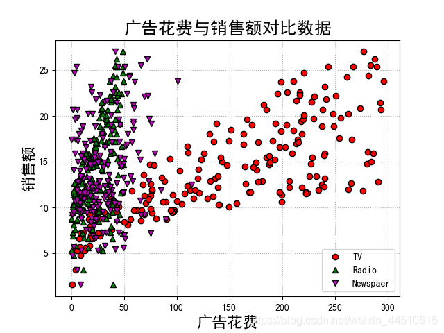

转载地址：https://maoli.blog.csdn.net/article/details/89457055 如侵犯您的版权，请留言回复原文章的地址，我们会给您删除此文章，给您带来不便请您谅解！