本文共 22808 字，大约阅读时间需要 76 分钟。

Datawhale 零基础入门数据挖掘-Task4 建模调参

四、建模与调参

Tip:此部分为零基础入门数据挖掘的 Task4 建模调参 部分，带你来了解各种模型以及模型的评价和调参策略，欢迎大家后续多多交流。

赛题：零基础入门数据挖掘 - 二手车交易价格预测

地址：https://tianchi.aliyun.com/competition/entrance/231784/introduction?spm=5176.12281957.1004.1.38b02448ausjSX

4.1 学习目标

• 了解常用的机器学习模型，并掌握机器学习模型的建模与调参流程
• 完成相应学习打卡任务

4.2 内容介绍

1. 线性回归模型：
   • 线性回归对于特征的要求；
   • 处理长尾分布；
   • 理解线性回归模型；
2. 模型性能验证：
   • 评价函数与目标函数；
   • 交叉验证方法；
   • 留一验证方法；
   • 针对时间序列问题的验证；
   • 绘制学习率曲线；
   • 绘制验证曲线；
3. 嵌入式特征选择：
   • Lasso回归；
   • Ridge回归；
   • 决策树；
4. 模型对比：
   • 常用线性模型；
   • 常用非线性模型；
5. 模型调参：
   • 贪心调参方法；
   • 网格调参方法；
   • 贝叶斯调参方法；

4.3 相关原理介绍与推荐

由于相关算法原理篇幅较长，本文推荐了一些博客与教材供初学者们进行学习。

4.3.1 线性回归模型

https://zhuanlan.zhihu.com/p/49480391

4.3.2 决策树模型

https://zhuanlan.zhihu.com/p/65304798

4.3.3 GBDT模型

https://zhuanlan.zhihu.com/p/45145899

4.3.4 XGBoost模型

https://zhuanlan.zhihu.com/p/86816771

4.3.5 LightGBM模型

https://zhuanlan.zhihu.com/p/89360721

4.3.6 推荐教材：

• 《机器学习》 https://book.douban.com/subject/26708119/
• 《统计学习方法》 https://book.douban.com/subject/10590856/
• 《Python大战机器学习》 https://book.douban.com/subject/26987890/
• 《面向机器学习的特征工程》 https://book.douban.com/subject/26826639/
• 《数据科学家访谈录》 https://book.douban.com/subject/30129410/

4.4 代码示例

4.4.1 读取数据

import pandas as pdimport numpy as npimport warningswarnings.filterwarnings('ignore')

reduce_mem_usage 函数通过调整数据类型，帮助我们减少数据在内存中占用的空间

def reduce_mem_usage(df):    """ iterate through all the columns of a dataframe and modify the data type        to reduce memory usage.            """    start_mem = df.memory_usage().sum()     print('Memory usage of dataframe is {:.2f} MB'.format(start_mem))        for col in df.columns:        col_type = df[col].dtype                if col_type != object:            c_min = df[col].min()            c_max = df[col].max()            if str(col_type)[:3] == 'int':                if c_min > np.iinfo(np.int8).min and c_max < np.iinfo(np.int8).max:                    df[col] = df[col].astype(np.int8)                elif c_min > np.iinfo(np.int16).min and c_max < np.iinfo(np.int16).max:                    df[col] = df[col].astype(np.int16)                elif c_min > np.iinfo(np.int32).min and c_max < np.iinfo(np.int32).max:                    df[col] = df[col].astype(np.int32)                elif c_min > np.iinfo(np.int64).min and c_max < np.iinfo(np.int64).max:                    df[col] = df[col].astype(np.int64)              else:                if c_min > np.finfo(np.float16).min and c_max < np.finfo(np.float16).max:                    df[col] = df[col].astype(np.float16)                elif c_min > np.finfo(np.float32).min and c_max < np.finfo(np.float32).max:                    df[col] = df[col].astype(np.float32)                else:                    df[col] = df[col].astype(np.float64)        else:            df[col] = df[col].astype('category')    end_mem = df.memory_usage().sum()     print('Memory usage after optimization is: {:.2f} MB'.format(end_mem))    print('Decreased by {:.1f}%'.format(100 * (start_mem - end_mem) / start_mem))    return df

sample_feature = reduce_mem_usage(pd.read_csv('data_for_tree.csv'))

Memory usage of dataframe is 60507328.00 MBMemory usage after optimization is: 15724107.00 MBDecreased by 74.0%

continuous_feature_names = [x for x in sample_feature.columns if x not in ['price','brand','model','brand']]

4.4.2 线性回归 & 五折交叉验证 & 模拟真实业务情况

sample_feature = sample_feature.dropna().replace('-', 0).reset_index(drop=True)sample_feature['notRepairedDamage'] = sample_feature['notRepairedDamage'].astype(np.float32)train = sample_feature[continuous_feature_names + ['price']]train_X = train[continuous_feature_names]train_y = train['price']

4.4.2 - 1 简单建模

from sklearn.linear_model import LinearRegression

model = LinearRegression(normalize=True)

model = model.fit(train_X, train_y)

查看训练的线性回归模型的截距（intercept）与权重(coef)

'intercept:'+ str(model.intercept_)sorted(dict(zip(continuous_feature_names, model.coef_)).items(), key=lambda x:x[1], reverse=True)

[('v_6', 3342612.384537345), ('v_8', 684205.534533214), ('v_9', 178967.94192530424), ('v_7', 35223.07319016895), ('v_5', 21917.550249749802), ('v_3', 12782.03250792227), ('v_12', 11654.925634146672), ('v_13', 9884.194615297649), ('v_11', 5519.182176035517), ('v_10', 3765.6101415594258), ('gearbox', 900.3205339198406), ('fuelType', 353.5206495542567), ('bodyType', 186.51797317460046), ('city', 45.17354204168846), ('power', 31.163045441455335), ('brand_price_median', 0.535967111869784), ('brand_price_std', 0.4346788365040235), ('brand_amount', 0.15308295553300566), ('brand_price_max', 0.003891831020467389), ('seller', -1.2684613466262817e-06), ('offerType', -4.759058356285095e-06), ('brand_price_sum', -2.2430642281682917e-05), ('name', -0.00042591632723759166), ('used_time', -0.012574429533889028), ('brand_price_average', -0.414105722833381), ('brand_price_min', -2.3163823428971835), ('train', -5.392535065078232), ('power_bin', -59.24591853031839), ('v_14', -233.1604256172217), ('kilometer', -372.96600915402496), ('notRepairedDamage', -449.29703564695365), ('v_0', -1490.6790578168238), ('v_4', -14219.648899108111), ('v_2', -16528.55239086934), ('v_1', -42869.43976200439)]

from matplotlib import pyplot as plt

subsample_index = np.random.randint(low=0, high=len(train_y), size=50)

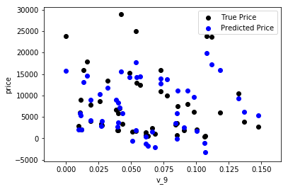
绘制特征v_9的值与标签的散点图，图片发现模型的预测结果（蓝色点）与真实标签（黑色点）的分布差异较大，且部分预测值出现了小于0的情况，说明我们的模型存在一些问题

plt.scatter(train_X['v_9'][subsample_index], train_y[subsample_index], color='black')plt.scatter(train_X['v_9'][subsample_index], model.predict(train_X.loc[subsample_index]), color='blue')plt.xlabel('v_9')plt.ylabel('price')plt.legend(['True Price','Predicted Price'],loc='upper right')print('The predicted price is obvious different from true price')plt.show()

The predicted price is obvious different from true price

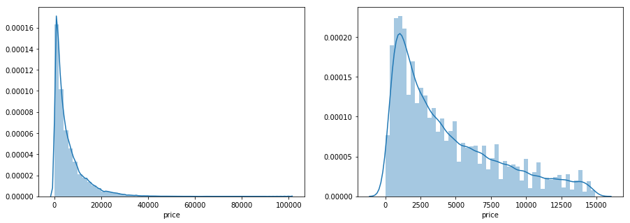
通过作图我们发现数据的标签（price）呈现长尾分布，不利于我们的建模预测。原因是很多模型都假设数据误差项符合正态分布，而长尾分布的数据违背了这一假设。参考博客：https://blog.csdn.net/Noob_daniel/article/details/76087829

import seaborn as snsprint('It is clear to see the price shows a typical exponential distribution')plt.figure(figsize=(15,5))plt.subplot(1,2,1)sns.distplot(train_y)plt.subplot(1,2,2)sns.distplot(train_y[train_y < np.quantile(train_y, 0.9)])

It is clear to see the price shows a typical exponential distribution
   

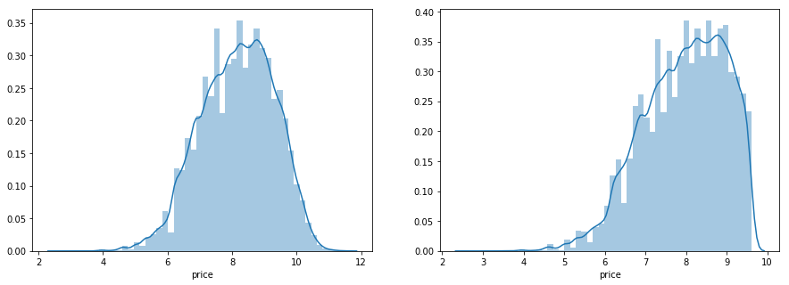
在这里我们对标签进行了 $log(x+1)$ 变换，使标签贴近于正态分布

train_y_ln = np.log(train_y + 1)

import seaborn as snsprint('The transformed price seems like normal distribution')plt.figure(figsize=(15,5))plt.subplot(1,2,1)sns.distplot(train_y_ln)plt.subplot(1,2,2)sns.distplot(train_y_ln[train_y_ln < np.quantile(train_y_ln, 0.9)])

The transformed price seems like normal distribution
   

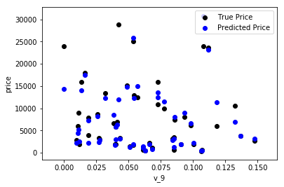
model = model.fit(train_X, train_y_ln)print('intercept:'+ str(model.intercept_))sorted(dict(zip(continuous_feature_names, model.coef_)).items(), key=lambda x:x[1], reverse=True)

intercept:23.515920686637713[('v_9', 6.043993029165403), ('v_12', 2.0357439855551394), ('v_11', 1.3607608712255672), ('v_1', 1.3079816298861897), ('v_13', 1.0788833838535354), ('v_3', 0.9895814429387444), ('gearbox', 0.009170812023421397), ('fuelType', 0.006447089787635784), ('bodyType', 0.004815242907679581), ('power_bin', 0.003151801949447194), ('power', 0.0012550361843629999), ('train', 0.0001429273782925814), ('brand_price_min', 2.0721302299502698e-05), ('brand_price_average', 5.308179717783439e-06), ('brand_amount', 2.8308531339942507e-06), ('brand_price_max', 6.764442596115763e-07), ('offerType', 1.6765966392995324e-10), ('seller', 9.308109838457312e-12), ('brand_price_sum', -1.3473184925468486e-10), ('name', -7.11403461065247e-08), ('brand_price_median', -1.7608143661053008e-06), ('brand_price_std', -2.7899058266986454e-06), ('used_time', -5.6142735899344175e-06), ('city', -0.0024992974087053223), ('v_14', -0.012754139659375262), ('kilometer', -0.013999175312751872), ('v_0', -0.04553774829634237), ('notRepairedDamage', -0.273686961116076), ('v_7', -0.7455902679730504), ('v_4', -0.9281349233755761), ('v_2', -1.2781892166433606), ('v_5', -1.5458846136756323), ('v_10', -1.8059217242413748), ('v_8', -42.611729973490604), ('v_6', -241.30992120503035)]

再次进行可视化，发现预测结果与真实值较为接近，且未出现异常状况

plt.scatter(train_X['v_9'][subsample_index], train_y[subsample_index], color='black')plt.scatter(train_X['v_9'][subsample_index], np.exp(model.predict(train_X.loc[subsample_index])), color='blue')plt.xlabel('v_9')plt.ylabel('price')plt.legend(['True Price','Predicted Price'],loc='upper right')print('The predicted price seems normal after np.log transforming')plt.show()

The predicted price seems normal after np.log transforming

4.4.2 - 2 五折交叉验证

在使用训练集对参数进行训练的时候，经常会发现人们通常会将一整个训练集分为三个部分（比如mnist手写训练集）。一般分为：训练集（train_set），评估集（valid_set），测试集（test_set）这三个部分。这其实是为了保证训练效果而特意设置的。其中测试集很好理解，其实就是完全不参与训练的数据，仅仅用来观测测试效果的数据。而训练集和评估集则牵涉到下面的知识了。

因为在实际的训练中，训练的结果对于训练集的拟合程度通常还是挺好的（初始条件敏感），但是对于训练集之外的数据的拟合程度通常就不那么令人满意了。因此我们通常并不会把所有的数据集都拿来训练，而是分出一部分来（这一部分不参加训练）对训练集生成的参数进行测试，相对客观的判断这些参数对训练集之外的数据的符合程度。这种思想就称为交叉验证（Cross Validation）

from sklearn.model_selection import cross_val_scorefrom sklearn.metrics import mean_absolute_error,  make_scorer

def log_transfer(func):    def wrapper(y, yhat):        result = func(np.log(y), np.nan_to_num(np.log(yhat)))        return result    return wrapper

scores = cross_val_score(model, X=train_X, y=train_y, verbose=1, cv = 5, scoring=make_scorer(log_transfer(mean_absolute_error)))

[Parallel(n_jobs=1)]: Using backend SequentialBackend with 1 concurrent workers.[Parallel(n_jobs=1)]: Done   5 out of   5 | elapsed:    1.1s finished

使用线性回归模型，对未处理标签的特征数据进行五折交叉验证（Error 1.36）

print('AVG:', np.mean(scores))

AVG: 1.3641908155886227

使用线性回归模型，对处理过标签的特征数据进行五折交叉验证（Error 0.19）

scores = cross_val_score(model, X=train_X, y=train_y_ln, verbose=1, cv = 5, scoring=make_scorer(mean_absolute_error))

[Parallel(n_jobs=1)]: Using backend SequentialBackend with 1 concurrent workers.[Parallel(n_jobs=1)]: Done   5 out of   5 | elapsed:    1.1s finished

print('AVG:', np.mean(scores))

AVG: 0.19382863663604424

scores = pd.DataFrame(scores.reshape(1,-1))scores.columns = ['cv' + str(x) for x in range(1, 6)]scores.index = ['MAE']scores

	cv1	cv2	cv3	cv4	cv5
MAE	0.191642	0.194986	0.192737	0.195329	0.19445

4.4.2 - 3 模拟真实业务情况

但在事实上，由于我们并不具有预知未来的能力，五折交叉验证在某些与时间相关的数据集上反而反映了不真实的情况。通过2018年的二手车价格预测2017年的二手车价格，这显然是不合理的，因此我们还可以采用时间顺序对数据集进行分隔。在本例中，我们选用靠前时间的4/5样本当作训练集，靠后时间的1/5当作验证集，最终结果与五折交叉验证差距不大

import datetime

sample_feature = sample_feature.reset_index(drop=True)

split_point = len(sample_feature) // 5 * 4

train = sample_feature.loc[:split_point].dropna()val = sample_feature.loc[split_point:].dropna()train_X = train[continuous_feature_names]train_y_ln = np.log(train['price'] + 1)val_X = val[continuous_feature_names]val_y_ln = np.log(val['price'] + 1)

model = model.fit(train_X, train_y_ln)

mean_absolute_error(val_y_ln, model.predict(val_X))

0.19443858353490887

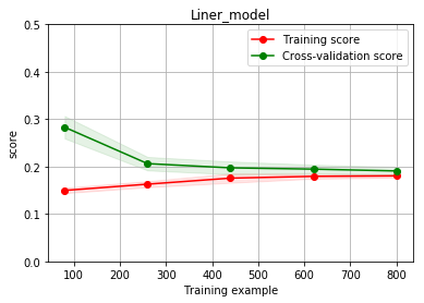
4.4.2 - 4 绘制学习率曲线与验证曲线

from sklearn.model_selection import learning_curve, validation_curve

? learning_curve

def plot_learning_curve(estimator, title, X, y, ylim=None, cv=None,n_jobs=1, train_size=np.linspace(.1, 1.0, 5 )):      plt.figure()      plt.title(title)      if ylim is not None:          plt.ylim(*ylim)      plt.xlabel('Training example')      plt.ylabel('score')      train_sizes, train_scores, test_scores = learning_curve(estimator, X, y, cv=cv, n_jobs=n_jobs, train_sizes=train_size, scoring = make_scorer(mean_absolute_error))      train_scores_mean = np.mean(train_scores, axis=1)      train_scores_std = np.std(train_scores, axis=1)      test_scores_mean = np.mean(test_scores, axis=1)      test_scores_std = np.std(test_scores, axis=1)      plt.grid()#区域      plt.fill_between(train_sizes, train_scores_mean - train_scores_std,                       train_scores_mean + train_scores_std, alpha=0.1,                       color="r")      plt.fill_between(train_sizes, test_scores_mean - test_scores_std,                       test_scores_mean + test_scores_std, alpha=0.1,                       color="g")      plt.plot(train_sizes, train_scores_mean, 'o-', color='r',               label="Training score")      plt.plot(train_sizes, test_scores_mean,'o-',color="g",               label="Cross-validation score")      plt.legend(loc="best")      return plt

plot_learning_curve(LinearRegression(), 'Liner_model', train_X[:1000], train_y_ln[:1000], ylim=(0.0, 0.5), cv=5, n_jobs=1)

4.4.3 多种模型对比

train = sample_feature[continuous_feature_names + ['price']].dropna()train_X = train[continuous_feature_names]train_y = train['price']train_y_ln = np.log(train_y + 1)

4.4.3 - 1 线性模型 & 嵌入式特征选择

本章节默认，学习者已经了解关于过拟合、模型复杂度、正则化等概念。否则请寻找相关资料或参考如下连接：

• 用简单易懂的语言描述「过拟合 overfitting」？ https://www.zhihu.com/question/32246256/answer/55320482
• 模型复杂度与模型的泛化能力 http://yangyingming.com/article/434/
• 正则化的直观理解 https://blog.csdn.net/jinping_shi/article/details/52433975

在过滤式和包裹式特征选择方法中，特征选择过程与学习器训练过程有明显的分别。而嵌入式特征选择在学习器训练过程中自动地进行特征选择。嵌入式选择最常用的是L1正则化与L2正则化。在对线性回归模型加入两种正则化方法后，他们分别变成了岭回归与Lasso回归。

from sklearn.linear_model import LinearRegressionfrom sklearn.linear_model import Ridgefrom sklearn.linear_model import Lasso

models = [LinearRegression(),          Ridge(),          Lasso()]

result = dict()for model in models:    model_name = str(model).split('(')[0]    scores = cross_val_score(model, X=train_X, y=train_y_ln, verbose=0, cv = 5, scoring=make_scorer(mean_absolute_error))    result[model_name] = scores    print(model_name + ' is finished')

LinearRegression is finishedRidge is finishedLasso is finished

对三种方法的效果对比

result = pd.DataFrame(result)result.index = ['cv' + str(x) for x in range(1, 6)]result

	LinearRegression	Ridge	Lasso
cv1	0.191642	0.195665	0.382708
cv2	0.194986	0.198841	0.383916
cv3	0.192737	0.196629	0.380754
cv4	0.195329	0.199255	0.385683
cv5	0.194450	0.198173	0.383555

model = LinearRegression().fit(train_X, train_y_ln)print('intercept:'+ str(model.intercept_))sns.barplot(abs(model.coef_), continuous_feature_names)

intercept:23.515984499017883
   

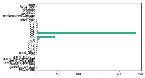
L2正则化在拟合过程中通常都倾向于让权值尽可能小，最后构造一个所有参数都比较小的模型。因为一般认为参数值小的模型比较简单，能适应不同的数据集，也在一定程度上避免了过拟合现象。可以设想一下对于一个线性回归方程，若参数很大，那么只要数据偏移一点点，就会对结果造成很大的影响；但如果参数足够小，数据偏移得多一点也不会对结果造成什么影响，专业一点的说法是『抗扰动能力强』

model = Ridge().fit(train_X, train_y_ln)print('intercept:'+ str(model.intercept_))sns.barplot(abs(model.coef_), continuous_feature_names)

intercept:5.901527844424091
   

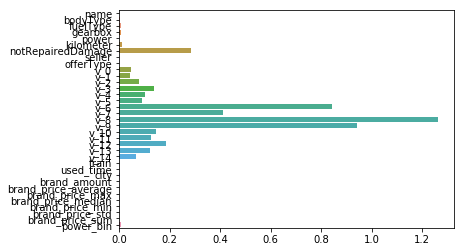
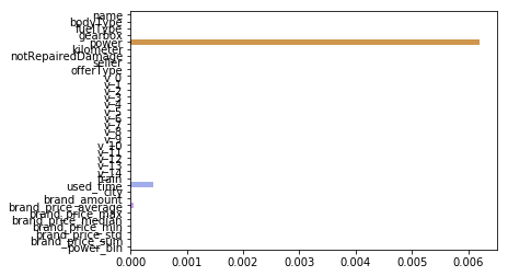
L1正则化有助于生成一个稀疏权值矩阵，进而可以用于特征选择。如下图，我们发现power与userd_time特征非常重要。

model = Lasso().fit(train_X, train_y_ln)print('intercept:'+ str(model.intercept_))sns.barplot(abs(model.coef_), continuous_feature_names)

intercept:8.674427764003347
   

除此之外，决策树通过信息熵或GINI指数选择分裂节点时，优先选择的分裂特征也更加重要，这同样是一种特征选择的方法。XGBoost与LightGBM模型中的model_importance指标正是基于此计算的

4.4.3 - 2 非线性模型

除了线性模型以外，还有许多我们常用的非线性模型如下，在此篇幅有限不再一一讲解原理。我们选择了部分常用模型与线性模型进行效果比对。

from sklearn.linear_model import LinearRegressionfrom sklearn.svm import SVCfrom sklearn.tree import DecisionTreeRegressorfrom sklearn.ensemble import RandomForestRegressorfrom sklearn.ensemble import GradientBoostingRegressorfrom sklearn.neural_network import MLPRegressorfrom xgboost.sklearn import XGBRegressorfrom lightgbm.sklearn import LGBMRegressor

models = [LinearRegression(),          DecisionTreeRegressor(),          RandomForestRegressor(),          GradientBoostingRegressor(),          MLPRegressor(solver='lbfgs', max_iter=100),           XGBRegressor(n_estimators = 100, objective='reg:squarederror'),           LGBMRegressor(n_estimators = 100)]

result = dict()for model in models:    model_name = str(model).split('(')[0]    scores = cross_val_score(model, X=train_X, y=train_y_ln, verbose=0, cv = 5, scoring=make_scorer(mean_absolute_error))    result[model_name] = scores    print(model_name + ' is finished')

LinearRegression is finishedDecisionTreeRegressor is finishedRandomForestRegressor is finishedGradientBoostingRegressor is finishedMLPRegressor is finishedXGBRegressor is finishedLGBMRegressor is finished

result = pd.DataFrame(result)result.index = ['cv' + str(x) for x in range(1, 6)]result

	LinearRegression	DecisionTreeRegressor	RandomForestRegressor	GradientBoostingRegressor	MLPRegressor	XGBRegressor	LGBMRegressor
cv1	0.191642	0.184566	0.136266	0.168626	124.299426	0.168698	0.141159
cv2	0.194986	0.187029	0.139693	0.171905	257.886236	0.172258	0.143363
cv3	0.192737	0.184839	0.136871	0.169553	236.829589	0.168604	0.142137
cv4	0.195329	0.182605	0.138689	0.172299	130.197264	0.172474	0.143461
cv5	0.194450	0.186626	0.137420	0.171206	268.090236	0.170898	0.141921

可以看到随机森林模型在每一个fold中均取得了更好的效果

4.4.4 模型调参

在此我们介绍了三种常用的调参方法如下：

• 贪心算法 https://www.jianshu.com/p/ab89df9759c8
• 网格调参 https://blog.csdn.net/weixin_43172660/article/details/83032029
• 贝叶斯调参 https://blog.csdn.net/linxid/article/details/81189154

## LGB的参数集合：objective = ['regression', 'regression_l1', 'mape', 'huber', 'fair']num_leaves = [3,5,10,15,20,40, 55]max_depth = [3,5,10,15,20,40, 55]bagging_fraction = []feature_fraction = []drop_rate = []

4.4.4 - 1 贪心调参

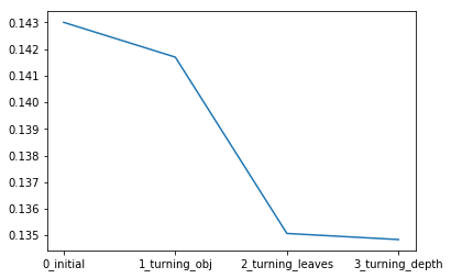
best_obj = dict()for obj in objective:    model = LGBMRegressor(objective=obj)    score = np.mean(cross_val_score(model, X=train_X, y=train_y_ln, verbose=0, cv = 5, scoring=make_scorer(mean_absolute_error)))    best_obj[obj] = score    best_leaves = dict()for leaves in num_leaves:    model = LGBMRegressor(objective=min(best_obj.items(), key=lambda x:x[1])[0], num_leaves=leaves)    score = np.mean(cross_val_score(model, X=train_X, y=train_y_ln, verbose=0, cv = 5, scoring=make_scorer(mean_absolute_error)))    best_leaves[leaves] = score    best_depth = dict()for depth in max_depth:    model = LGBMRegressor(objective=min(best_obj.items(), key=lambda x:x[1])[0],                          num_leaves=min(best_leaves.items(), key=lambda x:x[1])[0],                          max_depth=depth)    score = np.mean(cross_val_score(model, X=train_X, y=train_y_ln, verbose=0, cv = 5, scoring=make_scorer(mean_absolute_error)))    best_depth[depth] = score

sns.lineplot(x=['0_initial','1_turning_obj','2_turning_leaves','3_turning_depth'], y=[0.143 ,min(best_obj.values()), min(best_leaves.values()), min(best_depth.values())])

4.4.4 - 2 Grid Search 调参

from sklearn.model_selection import GridSearchCV

parameters = {
   'objective': objective , 'num_leaves': num_leaves, 'max_depth': max_depth}model = LGBMRegressor()clf = GridSearchCV(model, parameters, cv=5)clf = clf.fit(train_X, train_y)

clf.best_params_

{'max_depth': 15, 'num_leaves': 55, 'objective': 'regression'}

model = LGBMRegressor(objective='regression',                          num_leaves=55,                          max_depth=15)

np.mean(cross_val_score(model, X=train_X, y=train_y_ln, verbose=0, cv = 5, scoring=make_scorer(mean_absolute_error)))

0.13626164479243302

4.4.4 - 3 贝叶斯调参

from bayes_opt import BayesianOptimization

def rf_cv(num_leaves, max_depth, subsample, min_child_samples):    val = cross_val_score(        LGBMRegressor(objective = 'regression_l1',            num_leaves=int(num_leaves),            max_depth=int(max_depth),            subsample = subsample,            min_child_samples = int(min_child_samples)        ),        X=train_X, y=train_y_ln, verbose=0, cv = 5, scoring=make_scorer(mean_absolute_error)    ).mean()    return 1 - val

rf_bo = BayesianOptimization(    rf_cv,    {
       'num_leaves': (2, 100),    'max_depth': (2, 100),    'subsample': (0.1, 1),    'min_child_samples' : (2, 100)    })

rf_bo.maximize()

|   iter    |  target   | max_depth | min_ch... | num_le... | subsample |-------------------------------------------------------------------------| [0m 1       [0m | [0m 0.8649  [0m | [0m 89.57   [0m | [0m 47.3    [0m | [0m 55.13   [0m | [0m 0.1792  [0m || [0m 2       [0m | [0m 0.8477  [0m | [0m 99.86   [0m | [0m 60.91   [0m | [0m 15.35   [0m | [0m 0.4716  [0m || [95m 3       [0m | [95m 0.8698  [0m | [95m 81.74   [0m | [95m 83.32   [0m | [95m 92.59   [0m | [95m 0.9559  [0m || [0m 4       [0m | [0m 0.8627  [0m | [0m 90.2    [0m | [0m 8.754   [0m | [0m 43.34   [0m | [0m 0.7772  [0m || [0m 5       [0m | [0m 0.8115  [0m | [0m 10.07   [0m | [0m 86.15   [0m | [0m 4.109   [0m | [0m 0.3416  [0m || [95m 6       [0m | [95m 0.8701  [0m | [95m 99.15   [0m | [95m 9.158   [0m | [95m 99.47   [0m | [95m 0.494   [0m || [0m 7       [0m | [0m 0.806   [0m | [0m 2.166   [0m | [0m 2.416   [0m | [0m 97.7    [0m | [0m 0.224   [0m || [0m 8       [0m | [0m 0.8701  [0m | [0m 98.57   [0m | [0m 97.67   [0m | [0m 99.87   [0m | [0m 0.3703  [0m || [95m 9       [0m | [95m 0.8703  [0m | [95m 99.87   [0m | [95m 43.03   [0m | [95m 99.72   [0m | [95m 0.9749  [0m || [0m 10      [0m | [0m 0.869   [0m | [0m 10.31   [0m | [0m 99.63   [0m | [0m 99.34   [0m | [0m 0.2517  [0m || [95m 11      [0m | [95m 0.8703  [0m | [95m 52.27   [0m | [95m 99.56   [0m | [95m 98.97   [0m | [95m 0.9641  [0m || [0m 12      [0m | [0m 0.8669  [0m | [0m 99.89   [0m | [0m 8.846   [0m | [0m 66.49   [0m | [0m 0.1437  [0m || [0m 13      [0m | [0m 0.8702  [0m | [0m 68.13   [0m | [0m 75.28   [0m | [0m 98.71   [0m | [0m 0.153   [0m || [0m 14      [0m | [0m 0.8695  [0m | [0m 84.13   [0m | [0m 86.48   [0m | [0m 91.9    [0m | [0m 0.7949  [0m || [0m 15      [0m | [0m 0.8702  [0m | [0m 98.09   [0m | [0m 59.2    [0m | [0m 99.65   [0m | [0m 0.3275  [0m || [0m 16      [0m | [0m 0.87    [0m | [0m 68.97   [0m | [0m 98.62   [0m | [0m 98.93   [0m | [0m 0.2221  [0m || [0m 17      [0m | [0m 0.8702  [0m | [0m 99.85   [0m | [0m 63.74   [0m | [0m 99.63   [0m | [0m 0.4137  [0m || [0m 18      [0m | [0m 0.8703  [0m | [0m 45.87   [0m | [0m 99.05   [0m | [0m 99.89   [0m | [0m 0.3238  [0m || [0m 19      [0m | [0m 0.8702  [0m | [0m 79.65   [0m | [0m 46.91   [0m | [0m 98.61   [0m | [0m 0.8999  [0m || [0m 20      [0m | [0m 0.8702  [0m | [0m 99.25   [0m | [0m 36.73   [0m | [0m 99.05   [0m | [0m 0.1262  [0m || [0m 21      [0m | [0m 0.8702  [0m | [0m 85.51   [0m | [0m 85.34   [0m | [0m 99.77   [0m | [0m 0.8917  [0m || [0m 22      [0m | [0m 0.8696  [0m | [0m 99.99   [0m | [0m 38.51   [0m | [0m 89.13   [0m | [0m 0.9884  [0m || [0m 23      [0m | [0m 0.8701  [0m | [0m 63.29   [0m | [0m 97.93   [0m | [0m 99.94   [0m | [0m 0.9585  [0m || [0m 24      [0m | [0m 0.8702  [0m | [0m 93.04   [0m | [0m 71.42   [0m | [0m 99.94   [0m | [0m 0.9646  [0m || [0m 25      [0m | [0m 0.8701  [0m | [0m 99.73   [0m | [0m 16.21   [0m | [0m 99.38   [0m | [0m 0.9778  [0m || [0m 26      [0m | [0m 0.87    [0m | [0m 86.28   [0m | [0m 58.1    [0m | [0m 99.47   [0m | [0m 0.107   [0m || [0m 27      [0m | [0m 0.8703  [0m | [0m 47.28   [0m | [0m 99.83   [0m | [0m 99.65   [0m | [0m 0.4674  [0m || [0m 28      [0m | [0m 0.8703  [0m | [0m 68.29   [0m | [0m 99.51   [0m | [0m 99.4    [0m | [0m 0.2757  [0m || [0m 29      [0m | [0m 0.8701  [0m | [0m 76.49   [0m | [0m 73.41   [0m | [0m 99.86   [0m | [0m 0.9394  [0m || [0m 30      [0m | [0m 0.8695  [0m | [0m 37.27   [0m | [0m 99.87   [0m | [0m 89.87   [0m | [0m 0.7588  [0m |=========================================================================

1 - rf_bo.max['target']

0.1296693644053145

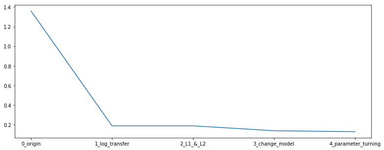
总结

在本章中，我们完成了建模与调参的工作，并对我们的模型进行了验证。此外，我们还采用了一些基本方法来提高预测的精度，提升如下图所示。

plt.figure(figsize=(13,5))sns.lineplot(x=['0_origin','1_log_transfer','2_L1_&_L2','3_change_model','4_parameter_turning'], y=[1.36 ,0.19, 0.19, 0.14, 0.13])

转载地址：https://blog.csdn.net/YYYYYJY/article/details/116034238 如侵犯您的版权，请留言回复原文章的地址，我们会给您删除此文章，给您带来不便请您谅解！