本文共 7661 字，大约阅读时间需要 25 分钟。

XGBoost输出特征重要性以及筛选特征

1，梯度提升算法是如何计算特征重要性的？

使用梯度提升算法的好处是在提升树被创建后，可以相对直接地得到每个属性的重要性得分。一般来说，重要性分数，衡量了特征在模型中的提升决策树构建中的价值。一个属性越多的被用来在模型中构建决策树，它的重要性就相对越高。

属性重要性是通过对数据集中的每个属性进行计算，并进行排序得到。在单个决策树中通过每个属性分裂点改进性能度量的量来计算属性重要性。由节点负责加权和记录次数，也就是说一个属性对分裂点改进性能度量越大（越靠近根节点），权值越大；被越多提升树所选择，属性越重要。性能度量可以是选择分裂节点的Gini纯度，也可以是其他度量函数。

最终将一个属性在所有提升树中的结果进行加权求和后然后平均，得到重要性得分。

2，绘制特征重要性

一个已训练的Xgboost模型能够自动计算特征重要性，这些重要性得分可以通过成员变量feature_importances_得到。可以通过如下命令打印：

print(model.feature_importances_)

我们可以直接在条形图上绘制这些分数，以便获得数据集中每个特征的相对重要性的直观显示，例如：

# plotpyplot.bar(range(len(model.feature_importances_)), model.feature_importances_)pyplot.show()

我们可以通过在the Pima Indians onset of diabetes 数据集上训练XGBoost模型来演示，并从计算的特征重要性中绘制条形图。

# plot feature importance manuallyfrom numpy import loadtxtfrom xgboost import XGBClassifierfrom matplotlib import pyplotfrom sklearn.datasets import load_iris# load datadataset = load_iris()# split data into X and yX = dataset.datay = dataset.target# fit model no training datamodel = XGBClassifier()model.fit(X, y)# feature importanceprint(model.feature_importances_)# plotpyplot.bar(range(len(model.feature_importances_)), model.feature_importances_)pyplot.show()

运行这个实例，首先输出特征重要性分数：

[0.17941953 0.11345647 0.41556728 0.29155672] 相对重要性条形图： 　　这种绘制的缺点在于，只显示了特征重要性而没有排序，可以在绘制之前对特征重要性得分进行排序。 　　通过内建的绘制函数进行特征重要性得分排序后的绘制，这个函数就是plot_importance()，示例如下：

# plot feature importance manuallyfrom numpy import loadtxtfrom xgboost import XGBClassifierfrom matplotlib import pyplotfrom sklearn.datasets import load_irisfrom xgboost import plot_importance # load datadataset = load_iris()# split data into X and yX = dataset.datay = dataset.target# fit model no training datamodel = XGBClassifier()model.fit(X, y)# feature importanceprint(model.feature_importances_)# plot feature importance plot_importance(model)pyplot.show()

示例得到条形图：

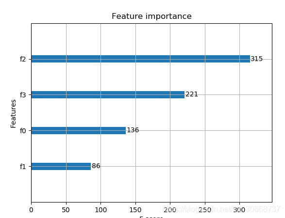
根据其在输入数组的索引，特征被自动命名为f0~f3，在问题描述中手动的将这些索引映射到名称，我们可以看到，f2具有最高的重要性，f1具有最低的重要性。

3，根据Xgboost特征重要性得分进行特征选择

特征重要性得分，可以用于在scikit-learn中进行特征选择。通过SelectFromModel类实现，该类采用模型并将数据集转换为具有选定特征的子集。这个类可以采取预先训练的模型，例如在整个数据集上训练的模型。然后，它可以阈值来决定选择哪些特征。当在SelectFromModel实例上调用transform()方法时，该阈值被用于在训练集和测试集上一致性选择相同特征。

在下面的示例中，我们首先在训练集上训练xgboost模型，然后在测试上评估。使用从训练数据集计算的特征重要性，然后，将模型封装在一个SelectFromModel实例中。我们使用这个来选择训练集上的特征，用所选择的特征子集训练模型，然后在相同的特征方案下对测试集进行评估。

# select features using thresholdselection = SelectFromModel(model, threshold=thresh, prefit=True)select_X_train = selection.transform(X_train)# train modelselection_model = XGBClassifier()selection_model.fit(select_X_train, y_train)# eval modelselect_X_test = selection.transform(X_test)y_pred = selection_model.predict(select_X_test)

我们可以通过测试多个阈值，来从特征重要性中选择特征。具体而言，每个输入变量的特征重要性，本质上允许我们通过重要性来测试每个特征子集。

完整代码如下：

# plot feature importance manuallyimport numpy as npfrom xgboost import XGBClassifierfrom matplotlib import pyplotfrom sklearn.datasets import load_irisfrom xgboost import plot_importancefrom sklearn.model_selection import train_test_splitfrom sklearn.metrics import accuracy_scorefrom sklearn.feature_selection import SelectFromModel # load datadataset = load_iris()# split data into X and yX = dataset.datay = dataset.target # split data into train and test setsX_train,X_test,y_train,y_test = train_test_split(X,y,test_size=0.33,random_state=7) # fit model no training datamodel = XGBClassifier()model.fit(X_train, y_train)# feature importanceprint(model.feature_importances_) # make predictions for test data and evaluatey_pred = model.predict(X_test)predictions = [round(value) for value in y_pred]accuracy = accuracy_score(y_test,predictions)print("Accuracy:%.2f%%"%(accuracy*100.0)) #fit model using each importance as a thresholdthresholds = np.sort(model.feature_importances_)for thresh in thresholds:    # select features using threshold    selection = SelectFromModel(model,threshold=thresh,prefit=True )    select_X_train = selection.transform(X_train)    # train model    selection_model = XGBClassifier()    selection_model.fit(select_X_train, y_train)    # eval model    select_X_test = selection.transform(X_test)    y_pred = selection_model.predict(select_X_test)    predictions = [round(value) for value in y_pred]    accuracy = accuracy_score(y_test,predictions)    print("Thresh=%.3f, n=%d, Accuracy: %.2f%%" % (thresh, select_X_train.shape[1], accuracy * 100.0))

运行示例，得到输出：

[0.20993228 0.09029345 0.54176074 0.15801354] Accuracy:92.00% Thresh=0.090, n=4, Accuracy: 92.00% Thresh=0.158, n=3, Accuracy: 92.00% Thresh=0.210, n=2, Accuracy: 86.00% Thresh=0.542, n=1, Accuracy: 90.00% 我们可以看到，模型的性能通常随着所选择的特征的数量减少，在这一问题上，可以对测试集准确率和模型复杂度做一个权衡，例如选择三个特征，接受准确率为92%，这可能是对这样一个小数据集的清洗，但是对于更大的数据集和使用交叉验证作为模型评估方案可能是更有用的策略。

4，网格搜索

代码1：

from sklearn.model_selection import GridSearchCVtuned_parameters= [{'n_estimators':[100,200,500],                  'max_depth':[3,5,7], ##range(3,10,2)                  'learning_rate':[0.5, 1.0],                  'subsample':[0.75,0.8,0.85,0.9]                  }]tuned_parameters= [{'n_estimators':[100,200,500,1000]                  }]clf = GridSearchCV(XGBClassifier(silent=0,nthread=4,learning_rate= 0.5,min_child_weight=1, max_depth=3,gamma=0,subsample=1,colsample_bytree=1,reg_lambda=1,seed=1000), param_grid=tuned_parameters,scoring='roc_auc',n_jobs=4,iid=False,cv=5) clf.fit(X_train, y_train)##clf.grid_scores_, clf.best_params_, clf.best_score_print(clf.best_params_)y_true, y_pred = y_test, clf.predict(X_test)print"Accuracy : %.4g" % metrics.accuracy_score(y_true, y_pred)y_proba=clf.predict_proba(X_test)[:,1]print "AUC Score (Train): %f" % metrics.roc_auc_score(y_true, y_proba)

代码2：

from sklearn.model_selection import GridSearchCVparameters= [{'learning_rate':[0.01,0.1,0.3],'n_estimators':[1000,1200,1500,2000,2500]}]clf = GridSearchCV(XGBClassifier(             max_depth=3,             min_child_weight=1,             gamma=0.5,             subsample=0.6,             colsample_bytree=0.6,             objective= 'binary:logistic', #逻辑回归损失函数             scale_pos_weight=1,             reg_alpha=0,             reg_lambda=1,             seed=27            ),            param_grid=parameters,scoring='roc_auc') clf.fit(X_train, y_train)print(clf.best_params_) y_pre= clf.predict(X_test)y_pro= clf.predict_proba(X_test)[:,1]print "AUC Score : %f" % metrics.roc_auc_score(y_test, y_pro)print"Accuracy : %.4g" % metrics.accuracy_score(y_test, y_pre)

输出特征重要性：

import pandas as pdimport matplotlib.pylab as pltfeat_imp = pd.Series(clf.booster().get_fscore()).sort_values(ascending=False)feat_imp.plot(kind='bar', title='Feature Importances')plt.ylabel('Feature Importance Score')plt.show()

补充：关于随机种子——random_state

random_state是一个随机种子，是在任意带有随机性的类或者函数里作为参数来控制随机模式。random_state取某一个值的时候，也就确定了一种规则。

random_state可以用于很多函数，比如训练集测试集的划分；构建决策树；构建随机森林

1，划分训练集和测试集的类train_test_split

随机数种子控制每次划分训练集和测试集的模式，其取值不变时划分得到的结果一模一样，其值改变时，划分得到的结果不同。若不设置此参数，则函数会自动选择一种随机模式，得到的结果也就不同。

2，构建决策树的函数

clf = tree.DecisionTreeClassifier(criterion="entropy",random_state=30,splitter="random")

其取值不变时，用相同的训练集建树得到的结果一模一样，对测试集的预测结果也是一样的

其取值改变时，得到的结果不同； 若不设置此参数（即设置为None），则函数会自动选择一种随机模式，每次得到的结果也就不同，可能稍微有所波动。

3，构建随机森林

clf = RandomForestClassifier(random_state=0)

其取值不变时，用相同的训练集建树得到的结果一模一样，对测试集的预测结果也是一样的

其取值改变时，得到的结果不同； 若不设置此参数（即设置为None），则函数会自动选择一种随机模式，每次得到的结果也就不同，可能稍微有所波动。

4，总结

在需要设置random_state的地方给其赋值，当多次运行此段代码得到完全一样的结果，别人运行代码也可以复现你的过程。若不设置此参数则会随机选择一个种子，执行结果也会因此不同。虽然可以对random_state进行调参，但是调参后再训练集上表现好的模型未必在陌生训练集上表现好，所以一般会随便选择一个random_state的值作为参数。

对于那些本质上是随机的过程，我们有必要控制随机的状态，这样才能重复的展现相同的结果。如果对随机状态不加控制，那么实验的结果就无法固定，而是随机的显示。 其实random_state 与 random seed作用是相同的，下面我们通过 random seed来学习一下 random_state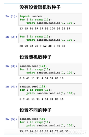： 第一段代码和第二段代码完全相同，在1~100中取10个随机数，都没有设置 random seed，它每次取的结果就不太，它的随机数种子与当前系统的时间有关。 第三段代码和第四段代码设置了相同的 random seed(123)，他们取的随机数就完全相同，你多运行几次也是这样。 第五段代码设置了 random seed(456)，但是与之前设置的不同，于是运行取随机数的结果也不同。

转载地址：https://blog.csdn.net/qq_30868737/article/details/108385115 如侵犯您的版权，请留言回复原文章的地址，我们会给您删除此文章，给您带来不便请您谅解！