本文共 4869 字，大约阅读时间需要 16 分钟。

（1）简介

 Deep Learning最简单的一种方法是利用人工神经网络的特点，人工神经网络（ANN）本身就是具有层次结构的系统，如果给定一个神经网络，我们假设其输出与输入是相同的，然后训练调整其参数，得到每一层中的权重。自然地，我们就得到了输入I的几种不同表示（每一层代表一种表示），这些表示就是特征。自动编码器就是一种尽可能复现输入信号的神经网络。为了实现这种复现，自动编码器就必须捕捉可以代表输入数据的最重要的因素，就像PCA那样，找到可以代表原信息的主要成分。

       具体过程简单的说明如下：

1）给定无标签数据，用非监督学习学习特征：

       在我们之前的神经网络中，如第一个图，我们输入的样本是有标签的，即（input, target），这样我们根据当前输出和target（label）之间的差去改变前面各层的参数，直到收敛。但现在我们只有无标签数据，也就是右边的图。那么这个误差怎么得到呢？

        如上图，我们将input输入一个encoder编码器，就会得到一个code，这个code也就是输入的一个表示，那么我们怎么知道这个code表示的就是input呢？我们加一个decoder解码器，这时候decoder就会输出一个信息，那么如果输出的这个信息和一开始的输入信号input是很像的（理想情况下就是一样的），那很明显，我们就有理由相信这个code是靠谱的。所以，我们就通过调整encoder和decoder的参数，使得重构误差最小，这时候我们就得到了输入input信号的第一个表示了，也就是编码code了。因为是无标签数据，所以误差的来源就是直接重构后与原输入相比得到。

（2）代码

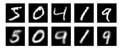
import torchimport torch.nn as nnimport torch.utils.data as Dataimport torchvisionimport matplotlib.pyplot as pltfrom mpl_toolkits.mplot3d import Axes3Dfrom matplotlib import cmimport numpy as np# torch.manual_seed(1)    # reproducible# Hyper ParametersEPOCH = 10BATCH_SIZE = 64LR = 0.005         # learning rateDOWNLOAD_MNIST = FalseN_TEST_IMG = 5# Mnist digits datasettrain_data = torchvision.datasets.MNIST(    root='./mnist/',    train=True,                                     # this is training data    transform=torchvision.transforms.ToTensor(),    # Converts a PIL.Image or numpy.ndarray to                                                    # torch.FloatTensor of shape (C x H x W) and normalize in the range [0.0, 1.0]    download=DOWNLOAD_MNIST,                        # download it if you don't have it)# plot one exampleprint(train_data.train_data.size())     # (60000, 28, 28)print(train_data.train_labels.size())   # (60000)plt.imshow(train_data.train_data[2].numpy(), cmap='gray')plt.title('%i' % train_data.train_labels[2])plt.show()# Data Loader for easy mini-batch return in training, the image batch shape will be (50, 1, 28, 28)train_loader = Data.DataLoader(dataset=train_data, batch_size=BATCH_SIZE, shuffle=True)class AutoEncoder(nn.Module):    def __init__(self):        super(AutoEncoder, self).__init__()        self.encoder = nn.Sequential(            nn.Linear(28*28, 128),            nn.Tanh(),            nn.Linear(128, 64),            nn.Tanh(),            nn.Linear(64, 12),            nn.Tanh(),            nn.Linear(12, 3),   # compress to 3 features which can be visualized in plt        )        self.decoder = nn.Sequential(            nn.Linear(3, 12),            nn.Tanh(),            nn.Linear(12, 64),            nn.Tanh(),            nn.Linear(64, 128),            nn.Tanh(),            nn.Linear(128, 28*28),            nn.Sigmoid(),       # compress to a range (0, 1)        )    def forward(self, x):        encoded = self.encoder(x)        decoded = self.decoder(encoded)        return encoded, decodedautoencoder = AutoEncoder()optimizer = torch.optim.Adam(autoencoder.parameters(), lr=LR)loss_func = nn.MSELoss()# initialize figuref, a = plt.subplots(2, N_TEST_IMG, figsize=(5, 2))plt.ion()   # continuously plot# original data (first row) for viewingview_data = train_data.train_data[:N_TEST_IMG].view(-1, 28*28).type(torch.FloatTensor)/255.for i in range(N_TEST_IMG):    a[0][i].imshow(np.reshape(view_data.data.numpy()[i], (28, 28)), cmap='gray'); a[0][i].set_xticks(()); a[0][i].set_yticks(())for epoch in range(EPOCH):    for step, (x, b_label) in enumerate(train_loader):        b_x = x.view(-1, 28*28)   # batch x, shape (batch, 28*28)        b_y = x.view(-1, 28*28)   # batch y, shape (batch, 28*28)        encoded, decoded = autoencoder(b_x)        loss = loss_func(decoded, b_y)      # mean square error        optimizer.zero_grad()               # clear gradients for this training step        loss.backward()                     # backpropagation, compute gradients        optimizer.step()                    # apply gradients        if step % 100 == 0:            print('Epoch: ', epoch, '| train loss: %.4f' % loss.data.numpy())            # plotting decoded image (second row)            _, decoded_data = autoencoder(view_data)            for i in range(N_TEST_IMG):                a[1][i].clear()                a[1][i].imshow(np.reshape(decoded_data.data.numpy()[i], (28, 28)), cmap='gray')                a[1][i].set_xticks(()); a[1][i].set_yticks(())            plt.draw(); plt.pause(0.05)plt.ioff()plt.show()# visualize in 3D plotview_data = train_data.train_data[:200].view(-1, 28*28).type(torch.FloatTensor)/255.encoded_data, _ = autoencoder(view_data)fig = plt.figure(2); ax = Axes3D(fig)X, Y, Z = encoded_data.data[:, 0].numpy(), encoded_data.data[:, 1].numpy(), encoded_data.data[:, 2].numpy()values = train_data.train_labels[:200].numpy()for x, y, z, s in zip(X, Y, Z, values):    c = cm.rainbow(int(255*s/9)); ax.text(x, y, z, s, backgroundcolor=c)ax.set_xlim(X.min(), X.max()); ax.set_ylim(Y.min(), Y.max()); ax.set_zlim(Z.min(), Z.max())plt.show()

（3）结果

注：代码主要参考：

       文章主要参考：

更多《计算机视觉与图形学》知识，可关注下方公众号：