本文共 23999 字，大约阅读时间需要 79 分钟。

# Pandas and numpy for data manipulationimport pandas as pdimport numpy as np# Modelingimport lightgbm as lgb# Evaluation of the modelfrom sklearn.model_selection import KFoldMAX_EVALS = 500N_FOLDS = 10

 

# Read in data and separate into training and testing setsdata = pd.read_csv('data/caravan-insurance-challenge.csv')train = data[data['ORIGIN'] == 'train']test = data[data['ORIGIN'] == 'test']# Extract the labels and format properlytrain_labels = np.array(train['CARAVAN'].astype(np.int32)).reshape((-1,))test_labels = np.array(test['CARAVAN'].astype(np.int32)).reshape((-1,))# Drop the unneeded columnstrain = train.drop(columns = ['ORIGIN', 'CARAVAN'])test = test.drop(columns = ['ORIGIN', 'CARAVAN'])# Convert to numpy array for splitting in cross validationfeatures = np.array(train)test_features = np.array(test)labels = train_labels[:]print('Train shape: ', train.shape)print('Test shape: ', test.shape)train.head()

 

 Distribution of Label

import matplotlib.pyplot as pltimport seaborn as sns%matplotlib inlineplt.hist(labels, edgecolor = 'k'); plt.xlabel('Label'); plt.ylabel('Count'); plt.title('Counts of Labels');

 

 

# Model with default hyperparametersmodel = lgb.LGBMClassifier()model

from sklearn.metrics import roc_auc_scorefrom timeit import default_timer as timerstart = timer()model.fit(features, labels)train_time = timer() - startpredictions = model.predict_proba(test_features)[:, 1]auc = roc_auc_score(test_labels, predictions)print('The baseline score on the test set is {:.4f}.'.format(auc))print('The baseline training time is {:.4f} seconds'.format(train_time))

 

# Hyperparameter gridparam_grid = {    'class_weight': [None, 'balanced'],    'boosting_type': ['gbdt', 'goss', 'dart'],    'num_leaves': list(range(30, 150)),    'learning_rate': list(np.logspace(np.log(0.005), np.log(0.2), base = np.exp(1), num = 1000)),    'subsample_for_bin': list(range(20000, 300000, 20000)),    'min_child_samples': list(range(20, 500, 5)),    'reg_alpha': list(np.linspace(0, 1)),    'reg_lambda': list(np.linspace(0, 1)),    'colsample_bytree': list(np.linspace(0.6, 1, 10))}# Subsampling (only applicable with 'goss')subsample_dist = list(np.linspace(0.5, 1, 100))

 

plt.hist(param_grid['learning_rate'], color = 'r', edgecolor = 'k');plt.xlabel('Learning Rate', size = 14); plt.ylabel('Count', size = 14); plt.title('Learning Rate Distribution', size = 18);

# Randomly sample parameters for gbmparams = {key: random.sample(value, 1)[0] for key, value in param_grid.items()}params

 

params['subsample'] = random.sample(subsample_dist, 1)[0] if params['boosting_type'] != 'goss' else 1.0params

 

# Create a lgb datasettrain_set = lgb.Dataset(features, label = labels)

 

# Perform cross validation with 10 foldsr = lgb.cv(params, train_set, num_boost_round = 10000, nfold = 10, metrics = 'auc',            early_stopping_rounds = 100, verbose_eval = False, seed = 50)# Highest scorer_best = np.max(r['auc-mean'])# Standard deviation of best scorer_best_std = r['auc-stdv'][np.argmax(r['auc-mean'])]print('The maximium ROC AUC on the validation set was {:.5f} with std of {:.5f}.'.format(r_best, r_best_std))print('The ideal number of iterations was {}.'.format(np.argmax(r['auc-mean']) + 1))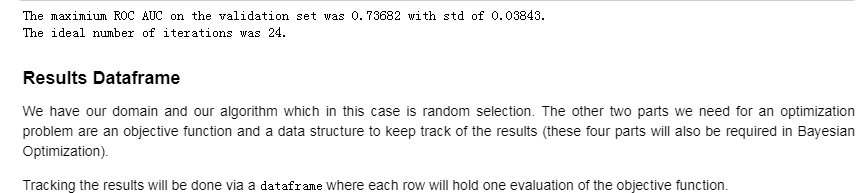

# Dataframe to hold cv resultsrandom_results = pd.DataFrame(columns = ['loss', 'params', 'iteration', 'estimators', 'time'],                       index = list(range(MAX_EVALS)))

def random_objective(params, iteration, n_folds = N_FOLDS):    """Random search objective function. Takes in hyperparameters       and returns a list of results to be saved."""    start = timer()        # Perform n_folds cross validation    cv_results = lgb.cv(params, train_set, num_boost_round = 10000, nfold = n_folds,                         early_stopping_rounds = 100, metrics = 'auc', seed = 50)    end = timer()    best_score = np.max(cv_results['auc-mean'])        # Loss must be minimized    loss = 1 - best_score        # Boosting rounds that returned the highest cv score    n_estimators = int(np.argmax(cv_results['auc-mean']) + 1)        # Return list of results    return [loss, params, iteration, n_estimators, end - start]

%%capturerandom.seed(50)# Iterate through the specified number of evaluationsfor i in range(MAX_EVALS):        # Randomly sample parameters for gbm    params = {key: random.sample(value, 1)[0] for key, value in param_grid.items()}        print(params)        if params['boosting_type'] == 'goss':        # Cannot subsample with goss        params['subsample'] = 1.0    else:        # Subsample supported for gdbt and dart        params['subsample'] = random.sample(subsample_dist, 1)[0]                    results_list = random_objective(params, i)        # Add results to next row in dataframe    random_results.loc[i, :] = results_list

 

# Sort results by best validation scorerandom_results.sort_values('loss', ascending = True, inplace = True)random_results.reset_index(inplace = True, drop = True)random_results.head()

# Find the best parameters and number of estimatorsbest_random_params = random_results.loc[0, 'params'].copy()best_random_estimators = int(random_results.loc[0, 'estimators'])best_random_model = lgb.LGBMClassifier(n_estimators=best_random_estimators, n_jobs = -1,                                        objective = 'binary', **best_random_params, random_state = 50)# Fit on the training databest_random_model.fit(features, labels)# Make test predictionspredictions = best_random_model.predict_proba(test_features)[:, 1]print('The best model from random search scores {:.4f} on the test data.'.format(roc_auc_score(test_labels, predictions)))print('This was achieved using {} search iterations.'.format(random_results.loc[0, 'iteration']))

 

import csvfrom hyperopt import STATUS_OKfrom timeit import default_timer as timerdef objective(params, n_folds = N_FOLDS):    """Objective function for Gradient Boosting Machine Hyperparameter Optimization"""        # Keep track of evals    global ITERATION        ITERATION += 1        # Retrieve the subsample if present otherwise set to 1.0    subsample = params['boosting_type'].get('subsample', 1.0)        # Extract the boosting type    params['boosting_type'] = params['boosting_type']['boosting_type']    params['subsample'] = subsample        # Make sure parameters that need to be integers are integers    for parameter_name in ['num_leaves', 'subsample_for_bin', 'min_child_samples']:        params[parameter_name] = int(params[parameter_name])        start = timer()        # Perform n_folds cross validation    cv_results = lgb.cv(params, train_set, num_boost_round = 10000, nfold = n_folds,                         early_stopping_rounds = 100, metrics = 'auc', seed = 50)        run_time = timer() - start        # Extract the best score    best_score = np.max(cv_results['auc-mean'])        # Loss must be minimized    loss = 1 - best_score        # Boosting rounds that returned the highest cv score    n_estimators = int(np.argmax(cv_results['auc-mean']) + 1)    # Write to the csv file ('a' means append)    of_connection = open(out_file, 'a')    writer = csv.writer(of_connection)    writer.writerow([loss, params, ITERATION, n_estimators, run_time])        # Dictionary with information for evaluation    return {'loss': loss, 'params': params, 'iteration': ITERATION,            'estimators': n_estimators,             'train_time': run_time, 'status': STATUS_OK}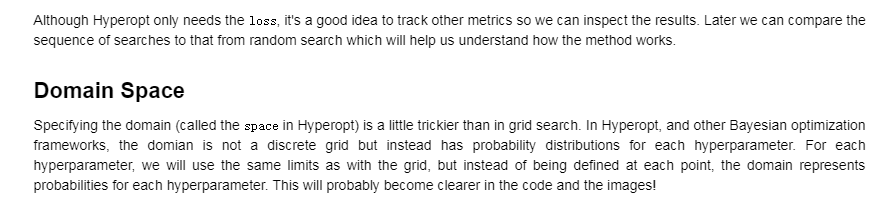

 

learning_rate_dist = []# Draw 10000 samples from the learning rate domainfor _ in range(10000):    learning_rate_dist.append(sample(learning_rate)['learning_rate'])    plt.figure(figsize = (8, 6))sns.kdeplot(learning_rate_dist, color = 'red', linewidth = 2, shade = True);plt.title('Learning Rate Distribution', size = 18); plt.xlabel('Learning Rate', size = 16); plt.ylabel('Density', size = 16);

 

 

# Discrete uniform distributionnum_leaves = {'num_leaves': hp.quniform('num_leaves', 30, 150, 1)}num_leaves_dist = []# Sample 10000 times from the number of leaves distributionfor _ in range(10000):    num_leaves_dist.append(sample(num_leaves)['num_leaves'])    # kdeplotplt.figure(figsize = (8, 6))sns.kdeplot(num_leaves_dist, linewidth = 2, shade = True);plt.title('Number of Leaves Distribution', size = 18); plt.xlabel('Number of Leaves', size = 16); plt.ylabel('Density', size = 16);

# boosting type domain boosting_type = {'boosting_type': hp.choice('boosting_type',                                             [{'boosting_type': 'gbdt', 'subsample': hp.uniform('subsample', 0.5, 1)},                                              {'boosting_type': 'dart', 'subsample': hp.uniform('subsample', 0.5, 1)},                                             {'boosting_type': 'goss', 'subsample': 1.0}])}# Draw a sampleparams = sample(boosting_type)params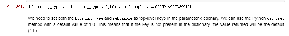

 

# Retrieve the subsample if present otherwise set to 1.0subsample = params['boosting_type'].get('subsample', 1.0)# Extract the boosting typeparams['boosting_type'] = params['boosting_type']['boosting_type']params['subsample'] = subsampleparams

 

# Define the search spacespace = {    'class_weight': hp.choice('class_weight', [None, 'balanced']),    'boosting_type': hp.choice('boosting_type', [{'boosting_type': 'gbdt', 'subsample': hp.uniform('gdbt_subsample', 0.5, 1)},                                                  {'boosting_type': 'dart', 'subsample': hp.uniform('dart_subsample', 0.5, 1)},                                                 {'boosting_type': 'goss', 'subsample': 1.0}]),    'num_leaves': hp.quniform('num_leaves', 30, 150, 1),    'learning_rate': hp.loguniform('learning_rate', np.log(0.01), np.log(0.2)),    'subsample_for_bin': hp.quniform('subsample_for_bin', 20000, 300000, 20000),    'min_child_samples': hp.quniform('min_child_samples', 20, 500, 5),    'reg_alpha': hp.uniform('reg_alpha', 0.0, 1.0),    'reg_lambda': hp.uniform('reg_lambda', 0.0, 1.0),    'colsample_bytree': hp.uniform('colsample_by_tree', 0.6, 1.0)}

 

# Sample from the full spacex = sample(space)# Conditional logic to assign top-level keyssubsample = x['boosting_type'].get('subsample', 1.0)x['boosting_type'] = x['boosting_type']['boosting_type']x['subsample'] = subsamplex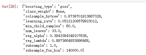

 

 

x = sample(space)subsample = x['boosting_type'].get('subsample', 1.0)x['boosting_type'] = x['boosting_type']['boosting_type']x['subsample'] = subsamplex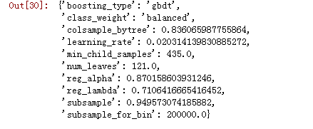

Optimization Algorithm

Although this is the most technical part of Bayesian optimization, defining the algorithm to use in Hyperopt is simple. We will use the Tree Parzen Estimator (read about it ) which is one method for constructing the surrogate function and choosing the next hyperparameters to evaluate.

from hyperopt import tpe# optimization algorithmtpe_algorithm = tpe.suggest

 

# File to save first resultsout_file = 'results/gbm_trials.csv'of_connection = open(out_file, 'w')writer = csv.writer(of_connection)# Write the headers to the filewriter.writerow(['loss', 'params', 'iteration', 'estimators', 'train_time'])of_connection.close()

 

 

from hyperopt import fmin

%%capture# Global variableglobal  ITERATIONITERATION = 0# Run optimizationbest = fmin(fn = objective, space = space, algo = tpe.suggest,             max_evals = MAX_EVALS, trials = bayes_trials, rstate = np.random.RandomState(50))

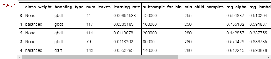
results = pd.read_csv('results/gbm_trials.csv')# Sort with best scores on top and reset index for slicingresults.sort_values('loss', ascending = True, inplace = True)results.reset_index(inplace = True, drop = True)results.head()

 

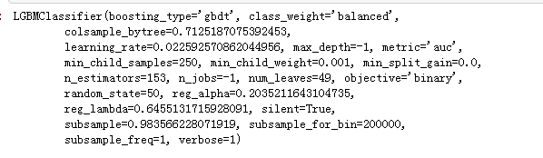
# Extract the ideal number of estimators and hyperparametersbest_bayes_estimators = int(results.loc[0, 'estimators'])best_bayes_params = ast.literal_eval(results.loc[0, 'params']).copy()# Re-create the best model and train on the training databest_bayes_model = lgb.LGBMClassifier(n_estimators=best_bayes_estimators, n_jobs = -1,                                        objective = 'binary', random_state = 50, **best_bayes_params)best_bayes_model.fit(features, labels)

# Evaluate on the testing data preds = best_bayes_model.predict_proba(test_features)[:, 1]print('The best model from Bayes optimization scores {:.5f} AUC ROC on the test set.'.format(roc_auc_score(test_labels, preds)))print('This was achieved after {} search iterations'.format(results.loc[0, 'iteration']))

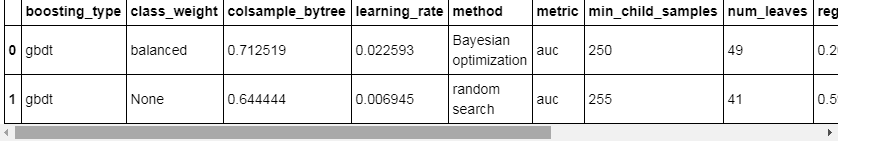
best_random_params['method'] = 'random search'best_bayes_params['method'] = 'Bayesian optimization'best_params = pd.DataFrame(best_bayes_params, index = [0]).append(pd.DataFrame(best_random_params, index = [0]),                                                                   ignore_index = True, sort = True)best_params

 

# Create a new dataframe for storing parametersrandom_params = pd.DataFrame(columns = list(random_results.loc[0, 'params'].keys()),                            index = list(range(len(random_results))))# Add the results with each parameter a different columnfor i, params in enumerate(random_results['params']):    random_params.loc[i, :] = list(params.values())    random_params['loss'] = random_results['loss']random_params['iteration'] = random_results['iteration']random_params.head()

 

# Create a new dataframe for storing parametersbayes_params = pd.DataFrame(columns = list(ast.literal_eval(results.loc[0, 'params']).keys()),                            index = list(range(len(results))))# Add the results with each parameter a different columnfor i, params in enumerate(results['params']):    bayes_params.loc[i, :] = list(ast.literal_eval(params).values())    bayes_params['loss'] = results['loss']bayes_params['iteration'] = results['iteration']bayes_params.head()

 

Learning Rates

The first plot shows the sampling distribution, random search, and Bayesian optimization learning rate distributions.

plt.figure(figsize = (20, 8))plt.rcParams['font.size'] = 18# Density plots of the learning rate distributions sns.kdeplot(learning_rate_dist, label = 'Sampling Distribution', linewidth = 2)sns.kdeplot(random_params['learning_rate'], label = 'Random Search', linewidth = 2)sns.kdeplot(bayes_params['learning_rate'], label = 'Bayes Optimization', linewidth = 2)plt.legend()plt.xlabel('Learning Rate'); plt.ylabel('Density'); plt.title('Learning Rate Distribution');

 

 

 

Boosting Type

Random search should use the boosting types with the same frequency. However, Bayesian Optimization might have decided (modeled) that one boosting type is better than another for this problem.

fig, axs = plt.subplots(1, 2, sharey = True, sharex = True)# Bar plots of boosting typerandom_params['boosting_type'].value_counts().plot.bar(ax = axs[0], figsize = (14, 6), color = 'orange', title = 'Random Search Boosting Type')bayes_params['boosting_type'].value_counts().plot.bar(ax = axs[1], figsize = (14, 6), color = 'green', title = 'Bayes Optimization Boosting Type');

 

print('Random Search boosting type percentages')100 * random_params['boosting_type'].value_counts() / len(random_params)

# Iterate through each hyperparameterfor i, hyper in enumerate(random_params.columns):    if hyper not in ['class_weight', 'boosting_type', 'iteration', 'subsample', 'metric', 'verbose']:        plt.figure(figsize = (14, 6))        # Plot the random search distribution and the bayes search distribution        if hyper != 'loss':            sns.kdeplot([sample(space[hyper]) for _ in range(1000)], label = 'Sampling Distribution')        sns.kdeplot(random_params[hyper], label = 'Random Search')        sns.kdeplot(bayes_params[hyper], label = 'Bayes Optimization')        plt.legend(loc = 1)        plt.title('{} Distribution'.format(hyper))        plt.xlabel('{}'.format(hyper)); plt.ylabel('Density');        plt.show();

 

 

 

The final graph shows that the validation loss for Bayesian Optimization tends to be lower than than from Random Search. This should give us confidence the method is working correctly. Again, this does not mean the hyperparameters found during Bayesian Optimization are necessarily better for the test set, only that they yield a lower loss in cross validation.

Evolution of Hyperparameters Searched

We can also plot the hyperparameters over time (against the number of iterations) to see how they change for the Bayes Optimization. First we will map the boosting_type to an integer for plotting.

# Map boosting type to integer (essentially label encoding)bayes_params['boosting_int'] = bayes_params['boosting_type'].replace({'gbdt': 1, 'goss': 2, 'dart': 3})# Plot the boosting type over the searchplt.plot(bayes_params['iteration'], bayes_params['boosting_int'], 'ro')plt.yticks([1, 2, 3], ['gdbt', 'goss', 'dart']);plt.xlabel('Iteration'); plt.title('Boosting Type over Search');

 

fig, axs = plt.subplots(1, 4, figsize = (24, 6))i = 0# Plot of four hyperparametersfor i, hyper in enumerate(['colsample_bytree', 'learning_rate', 'min_child_samples', 'num_leaves']):            # Scatterplot        sns.regplot('iteration', hyper, data = bayes_params, ax = axs[i])        axs[i].set(xlabel = 'Iteration', ylabel = '{}'.format(hyper), title = '{} over Search'.format(hyper));plt.tight_layout()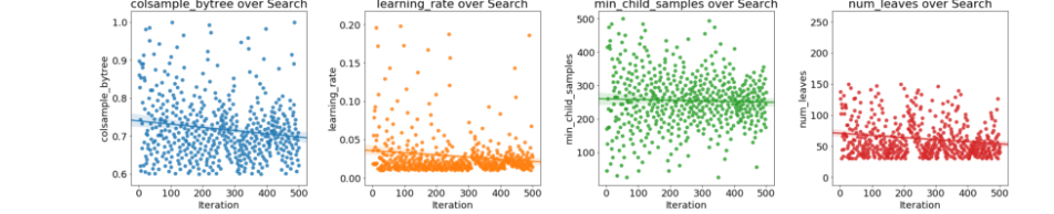

fig, axs = plt.subplots(1, 3, figsize = (18, 6))i = 0# Scatterplot of next three hyperparametersfor i, hyper in enumerate(['reg_alpha', 'reg_lambda', 'subsample_for_bin']):        sns.regplot('iteration', hyper, data = bayes_params, ax = axs[i])        axs[i].set(xlabel = 'Iteration', ylabel = '{}'.format(hyper), title = '{} over Search'.format(hyper));plt.tight_layout()

 

 

If there are trends in these plots, we can use them to inform subsequent searches. We might even want to use grid search focusing on a much smaller region of hyperparameter space based on the Bayesian Optimization results.

Validation Losses

Finally, we can look at the losses recorded by both random search and Bayes Optimization. We would expect the average loss recorded by Bayes Optimization to be lower because this method should spend more time in promising regions of the search space.

# Dataframe of just scoresscores = pd.DataFrame({'ROC AUC': 1 - random_params['loss'], 'iteration': random_params['iteration'], 'search': 'random'})scores = scores.append(pd.DataFrame({'ROC AUC': 1 - bayes_params['loss'], 'iteration': bayes_params['iteration'], 'search': 'Bayes'}))scores['ROC AUC'] = scores['ROC AUC'].astype(np.float32)scores['iteration'] = scores['iteration'].astype(np.int32)scores.head()

plt.figure(figsize = (18, 6))# Random search scoresplt.subplot(1, 2, 1)plt.hist(1 - random_results['loss'].astype(np.float64), label = 'Random Search', edgecolor = 'k');plt.xlabel("Validation ROC AUC"); plt.ylabel("Count"); plt.title("Random Search Validation Scores")plt.xlim(0.75, 0.78)# Bayes optimization scoresplt.subplot(1, 2, 2)plt.hist(1 - bayes_params['loss'], label = 'Bayes Optimization', edgecolor = 'k');plt.xlabel("Validation ROC AUC"); plt.ylabel("Count"); plt.title("Bayes Optimization Validation Scores");plt.xlim(0.75, 0.78);

 

It's reassuring to see that the validation ROC AUC scores of Bayesian optimization increase over time. What this shows is that the model is exploring hyperparameters that are better according to the cross validation metric! It would be interesting to continue searching and see if there is a plateau in the validation scores (there would have to be eventually). Moreover, even if validation scores continue to increase, that does not mean a better model for the testing data!

If we want to save to save the trials results, we can use the json format.

import json# Save the trial resultswith open('results/trials.json', 'w') as f:    f.write(json.dumps(bayes_trials.results))

 

# Save dataframes of parametersbayes_params.to_csv('results/bayes_params.csv', index = False)random_params.to_csv('results/random_params.csv', index = False)

%capture# Use the same trials object to keep trainingbest = fmin(fn = objective, space = space, algo = tpe.suggest,             max_evals = MAX_EVALS, trials = bayes_trials, verbose = 1, rstate = np.random.RandomState(50))

 

# Sort the trials with lowest loss (highest AUC) firstbayes_trials_results = sorted(bayes_trials.results, key = lambda x: x['loss'])bayes_trials_results[:2]

results = pd.read_csv('results/gbm_trials.csv')# Sort values with best on top and reset index for slicingresults.sort_values('loss', ascending = True, inplace = True)results.reset_index(inplace = True, drop = True)results.head()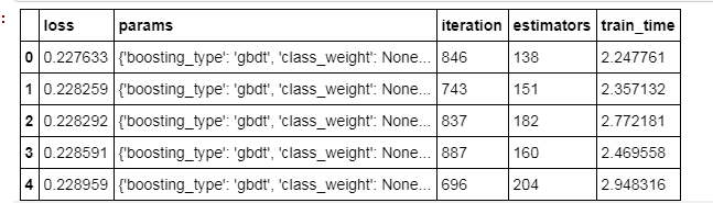

 

# Extract the ideal number of estimators and hyperparametersbest_bayes_estimators = int(results.loc[0, 'estimators'])best_bayes_params = ast.literal_eval(results.loc[0, 'params']).copy()# Re-create the best model and train on the training databest_bayes_model = lgb.LGBMClassifier(n_estimators=best_bayes_estimators, n_jobs = -1,                                        objective = 'binary', random_state = 50, **best_bayes_params)best_bayes_model.fit(features, labels)

 

LGBMClassifier(boosting_type='gbdt', class_weight=None,        colsample_bytree=0.6311794044268164,        learning_rate=0.027802518491219938, max_depth=-1, metric='auc',        min_child_samples=250, min_child_weight=0.001, min_split_gain=0.0,        n_estimators=138, n_jobs=-1, num_leaves=40, objective='binary',        random_state=50, reg_alpha=0.06183118355912668,        reg_lambda=0.24742831407472365, silent=True,        subsample=0.999742610271968, subsample_for_bin=280000,        subsample_freq=1, verbose=1)

# Evaluate on the testing data preds = best_bayes_model.predict_proba(test_features)[:, 1]print('The best model from Bayes optimization scores {:.5f} AUC ROC on the test set.'.format(roc_auc_score(test_labels, preds)))print('This was achieved after {} search iterations'.format(results.loc[0, 'iteration']))

The best model from Bayes optimization scores 0.72736 AUC ROC on the test set.This was achieved after 846 search iterations

The continuation of the search did slightly improve the validation score (again depending on training run). Instead of training more, we might want to restart the search so the algorithm can spend more time exploring the domain space. As searching continues, the algorithm shifts from exploring (trying new values) to exploiting (trying those values that worked best in the past). This is generally what we want unless the model gets stuck in a local minimum at which point we would want to restart the search in a different region of the hyperparameter space. Bayesian Optimization of hyperparameters is still prone to overfitting, even when using cross-validation because it can get settle into a local minimum of the objective function. It is very difficult to tell when this occurs for a high-dimensional problem!

Conclusions

In this notebook, we saw how to implement automated hyperparameter tuning with Bayesian Optimization methods. We used the open-source Python library Hyperopt with the Tree Parzen Estimator to optimize the hyperparameters of a gradient boosting machine.

Bayesian model-based optimization can be more efficient than random search, finding a better set of model hyperparameters in fewer search iterations (although not in every case). However, just because the model hyperparameters are better on the validation set does not mean they are better for the testing set! For this training run, Bayesian Optimization found a better set of hyperparamters according to the validation and the test data although the testing score was much lower than the validation ROC AUC. This is a useful lesson that even when using cross-validation, overfitting is still one of the top problems in machine learning.

Bayesian optimization is a powerful technique that we can use to tune any machine learning model, so long as we can define an objective function that returns a value to minimize and a domain space over which to search. This can extend to any function that we want to minimize (not just hyperparameter tuning). Bayesian optimization can be a significant upgrade over uninformed methods such as random search and because of the ease of use in Python are now a good option to use for hyperparameter tuning. As with most subjects in machine learning, there is no single best answer for hyperparameter tuning, but Bayesian optimization methods should be a tool that helps data scientists with the tedious but necessary task of model tuning!