本文共 10088 字，大约阅读时间需要 33 分钟。

许多机器学习问题需要从 类别变量、文本、图片中学习，需要从中提取出数字特征

1. 从类别变量中提取特征

通常使用 one-hot 编码，产生2进制的编码，会扩展数据，当数据值种类多时，不宜使用

from sklearn.feature_extraction import DictVectorizeronehot_encoder = DictVectorizer()X=[    {
   'city':'Beijing'},    {
   'city':'Guangzhou'},    {
   'city':'Shanghai'}]print(onehot_encoder.fit_transform(X).toarray())

[[1. 0. 0.] [0. 1. 0.] [0. 0. 1.]]

one-hot 编码，没有顺序或大小之分，相比于用 0， 1， 2 来表示上述 3 个city，one-hot编码更好

• ，如果分类变量是数字类型，请使用

this transformer will only do a binary one-hot encoding when feature values are of type string.

If categorical features are represented as numeric values such as int, the DictVectorizer can be followed by sklearn.preprocessing.OneHotEncoder to complete binary one-hot encoding.

• DictVectorizer 对数字特征 失效案列：

X=[    {
   'city':1},    {
   'city':4},    {
   'city':5}]onehot_encoder = DictVectorizer()print(onehot_encoder.fit_transform(X).toarray())

[[1.] [4.] [5.]]

• OneHotEncoder 既可针对 string 类型，也可以对数字类型，进行编码

# string 类型from sklearn.preprocessing import OneHotEncoderimport pandas as pdonehot_encoder = OneHotEncoder()X=[    {
   'city':'Beijing'},    {
   'city':'Guangzhou'},    {
   'city':'Shanghai'}]X = pd.DataFrame(X)print(onehot_encoder.fit_transform(X).toarray())

[[1. 0. 0.] [0. 1. 0.] [0. 0. 1.]]

# 数字类型onehot_encoder = OneHotEncoder()X=[    {
   'city':1},    {
   'city':4},    {
   'city':5}]X = pd.DataFrame(X)print(onehot_encoder.fit_transform(X).toarray())

[[1. 0. 0.] [0. 1. 0.] [0. 0. 1.]]

2. 特征标准化

• 防止特征淹没，某些特征无法发挥作用
• 加快算法收敛

from sklearn import preprocessingimport numpy as npX = np.array([    [0., 0., 5., 13., 9., 1.],    [0., 0., 13., 15., 10., 15.],    [0., 3., 15., 2., 0., 11.]])s = preprocessing.StandardScaler()print(s.fit_transform(X))

StandardScaler 均值为0，方差为1

[[ 0.         -0.70710678 -1.38873015  0.52489066  0.59299945 -1.35873244] [ 0.         -0.70710678  0.46291005  0.87481777  0.81537425  1.01904933] [ 0.          1.41421356  0.9258201  -1.39970842 -1.4083737   0.33968311]]

RobustScaler 对异常值有更好的鲁棒性，减轻异常值的影响

This Scaler removes the median and scales the data according to the quantile range (defaults to IQR: Interquartile Range).

The IQR is the range between the 1st quartile (25th quantile) and the 3rd quartile (75th quantile).

from sklearn.preprocessing import RobustScalers = RobustScaler()print(s.fit_transform(X))

[[ 0.          0.         -1.6         0.          0.         -1.42857143] [ 0.          0.          0.          0.30769231  0.2         0.57142857] [ 0.          2.          0.4        -1.69230769 -1.8         0.        ]]

3. 从文本中提取特征

文本通常为自然语言

3.1 词袋模型

• 不会编码任何文本句法，忽略单词顺序，忽略语法，忽略词频
• 可看做 one-hot 的一种扩展，会对文本中关注的每一个单词创建一个特征
• 可用于文档分类和检索

corpus = [    "UNC played Duke in basketball",    "Duke lost the basketball game"]from sklearn.feature_extraction.text import CountVectorizervectorizer = CountVectorizer()print(vectorizer.fit_transform(corpus).todense())# [[1 1 0 1 0 1 0 1]# [1 1 1 0 1 0 1 0]]print(vectorizer.vocabulary_)# {'unc': 7, 'played': 5, 'duke': 1, 'in': 3, #  'basketball': 0, 'lost': 4, 'the': 6, 'game': 2}

• 注意：只会提取长度 >= 2 的单词，添加一个句子，该句子的单词 I，a 没有向量化

corpus.append("I ate a sandwich and an apple")print(vectorizer.fit_transform(corpus).todense())# [[0 0 0 0 1 1 0 1 0 1 0 0 1]#  [0 0 0 0 1 1 1 0 1 0 0 1 0]#  [1 1 1 1 0 0 0 0 0 0 1 0 0]]print(vectorizer.vocabulary_)# {'unc': 12, 'played': 9, 'duke': 5, 'in': 7, #  'basketball': 4, 'lost': 8, 'the': 11, 'game': 6, #  'ate': 3, 'sandwich': 10, 'and': 1, 'an': 0, 'apple': 2}

• 进行文本相似度计算，计算文本向量之间的欧氏距离（L₂范数）

from sklearn.metrics.pairwise import euclidean_distancesX = vectorizer.fit_transform(corpus).todense()print("distance between doc1 and doc2 ", euclidean_distances(X[0],X[1]))print("distance between doc1 and doc3 ", euclidean_distances(X[0],X[2]))print("distance between doc2 and doc3 ", euclidean_distances(X[1],X[2]))# distance between doc1 and doc2  [[2.44948974]]# distance between doc1 and doc3  [[3.16227766]]# distance between doc2 and doc3  [[3.16227766]]

可以看出，文档1跟文档2更相似

3.2 停用词过滤

降维策略：

• 所有单词转成小写，对单词的意思没有影响
• 忽略语料库中大部分文档中经常出现的单词，如the\a\an\do \be\will\on\around等，称之 stop_words
• CountVectorizer 可以通过 stop_words 关键词参数，过滤停用词，它本身也有一个基本的英语停用词列表

vectorizer = CountVectorizer(stop_words='english')print(vectorizer.fit_transform(corpus).todense())# [[0 0 1 1 0 0 1 0 1]#  [0 0 1 1 1 1 0 0 0]#  [1 1 0 0 0 0 0 1 0]]print(vectorizer.vocabulary_)# {'unc': 8, 'played': 6, 'duke': 3, 'basketball': 2, # 'lost': 5, 'game': 4, 'ate': 1, 'sandwich': 7, 'apple': 0}

我们发现 in\the\and\an不见了

3.3 词干提取和词形还原

停用词列表包含的词很少，过滤后依然包含很多单词怎么办？

• 词干提取、词形还原，进一步降维

例如，jumping\jumps\jump，一篇报道跳远比赛的文章中，这几个词时分别编码的，我们可以对他们进行统一处理，压缩成单个特征

corpus = [    'He ate the sandwiches',    'Every sandwich was eaten by him']vectorizer = CountVectorizer(binary=True, stop_words='english')print(vectorizer.fit_transform(corpus).todense())# [[1 0 1 0]# [0 1 0 1]]print(vectorizer.vocabulary_)# {'ate': 0, 'sandwiches': 2, 'sandwishes': 3, 'eaten': 1}

我们看到这两个句子表达的一个意思，特征向量却没有一个共同元素

• Lemmatizer 词性还原
  注：，解压、添加路径、重新打开python即可

corpus = [    'I am gathering ingredients for the sandwich.',    'There were many peoples at the gathering.']from nltk.stem.wordnet import WordNetLemmatizer# help(WordNetLemmatizer)lemmatizer = WordNetLemmatizer()print(lemmatizer.lemmatize('gathering','v')) # gather，动词print(lemmatizer.lemmatize('gathering','n')) # gathering，名词

• PorterStemmer 词干提取

from nltk.stem import PorterStemmer# help(PorterStemmer)stemmer = PorterStemmer()print(stemmer.stem('gathering')) # gather

小例子：

from nltk import word_tokenize # 取词from nltk.stem import PorterStemmer # 词干提取from nltk.stem.wordnet import WordNetLemmatizer # 词性还原from nltk import pos_tag # 词性标注wordnet_tags = ['n','v']corpus = [    'He ate the sandwiches',    'Every sandwich was eaten by him']stemmer = PorterStemmer()print("词干：", [[stemmer.stem(word) for word in word_tokenize(doc)] 												 for doc in corpus])# 词干： [['He', 'ate', 'the', 'sandwich'], #		['everi', 'sandwich', 'wa', 'eaten', 'by', 'him']]

def lemmatize(word, tag):    if tag[0].lower() in ['n','v']:        return lemmatizer.lemmatize(word, tag[0].lower())    return wordlemmatizer = WordNetLemmatizer()tagged_corpus = [pos_tag(word_tokenize(doc)) for doc in corpus]print(tagged_corpus)# [[('He', 'PRP'), ('ate', 'VBD'), ('the', 'DT'), ('sandwiches', 'NNS')], #  [('Every', 'DT'), ('sandwich', 'NN'), ('was', 'VBD'), #   ('eaten', 'VBN'), ('by', 'IN'), ('him', 'PRP')]]print('词性还原：',[[lemmatize(word,tag) for word, tag in doc] for doc in tagged_corpus])# 词性还原： [['He', 'eat', 'the', 'sandwich'], #            ['Every', 'sandwich', 'be', 'eat', 'by', 'him']]对 n,v 开头的词性的单词进行了词性还原

3.4 TF-IDF 权重扩展词包

词频是很重要的，创建编码单词频数的特征向量

import numpy as npfrom sklearn.feature_extraction.text import CountVectorizercorpus = ["The dog ate a sandwich, the people manufactured many sandwiches,\          and I ate a sandwich"]          vectorizer = CountVectorizer(stop_words='english')freq = np.array(vectorizer.fit_transform(corpus).todense())freq # array([[2, 1, 1, 3]], dtype=int64)vectorizer.vocabulary_#  {'dog': 1, 'ate': 0, 'sandwich': 3, 'people': 2}for word, idx in vectorizer.vocabulary_.items():    print(word, " 出现了 ", freq[0][idx]," 次")

dog  出现了  1  次ate  出现了  2  次sandwich  出现了  2  次people  出现了  1  次manufactured  出现了  1  次sandwiches  出现了  1  次

• sklearn 的TfidfVectorizer 可以统计单词的权值：单词频率-逆文本频率 TF-IDF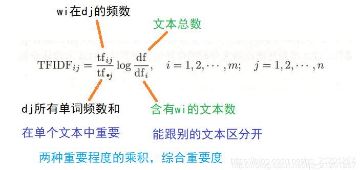
  

from sklearn.feature_extraction.text import TfidfVectorizercorpus = ["The dog ate a sandwich, and I ate a sandwich",          "the people manufactured a sandwich"]vectorizer = TfidfVectorizer(stop_words='english')print(vectorizer.fit_transform(corpus).todense())print(vectorizer.vocabulary_)

[[0.75458397 0.37729199 0.         0.         0.53689271] [0.         0.         0.6316672  0.6316672  0.44943642]]{
   'dog': 1, 'ate': 0, 'sandwich': 4, 'people': 3, 'manufactured': 2}

3.5 空间有效特征向量化与哈希技巧

• 书上大概意思是说可以省内存，可以用于在线流式任务创建特征向量

from sklearn.feature_extraction.text import HashingVectorizer# help(HashingVectorizer)corpus = [     'This is the first document.',     'This document is the second document.' ]vectorizer = HashingVectorizer(n_features=2**4)X = vectorizer.fit_transform(corpus).todense()print(X)x = vectorizer.transform(['This is the first document.']).todense()print(x)x in X # True

[[-0.57735027  0.          0.          0.          0.          0.   0.          0.         -0.57735027  0.          0.          0.   0.          0.57735027  0.          0.        ] [-0.81649658  0.          0.          0.          0.          0.   0.          0.          0.          0.          0.          0.40824829   0.          0.40824829  0.          0.        ]][[-0.57735027  0.          0.          0.          0.          0.   0.          0.         -0.57735027  0.          0.          0.   0.          0.57735027  0.          0.        ]]

3.6 词向量

词向量模型相比于词袋模型更好些。

词向量模型在类似的词语上产生类似的词向量（如，small、tiny都表示小），反义词的向量则只在很少的几个维度类似

# google colab 运行以下代码import gensimfrom google.colab import drivedrive.mount('/gdrive')# !git clone https://github.com/mmihaltz/word2vec-GoogleNews-vectors.git! wget -c "https://s3.amazonaws.com/dl4j-distribution/GoogleNews-vectors-negative300.bin.gz"!cd /content!gzip -d /content/GoogleNews-vectors-negative300.bin.gzmodel = gensim.models.KeyedVectors.load_word2vec_format('/content/GoogleNews-vectors-negative300.bin', binary=True)

embedding = model.word_vec('cat')embedding.shape  # (300,)相似度print(model.similarity('cat','dog'))  # 0.76094574print(model.similarity('cat','sandwich'))  # 0.17211203最相似的n个单词print(model.most_similar(positive=['good','ok'],negative=['bad'],topn=3))# [('okay', 0.7390689849853516), #  ('alright', 0.7239435911178589), #  ('OK', 0.5975555777549744)]

4. 从图像中提取特征

4.1 从像素强度中提取特征

将图片的矩阵展平后作为特征向量

• 有缺点，产出的模型对缩放、旋转、平移很敏感，对光照强度变化也很敏感

from sklearn import datasetsdigits = datasets.load_digits()print(digits.images[0].reshape(-1,64))

图片特征向量[[ 0.  0.  5. 13.  9.  1.  0.  0.  0.  0. 13. 15. 10. 15.  5.  0.  0.  3.  15.  2.  0. 11.  8.  0.  0.  4. 12.  0.  0.  8.  8.  0.  0.  5.  8.  0.   0.  9.  8.  0.  0.  4. 11.  0.  1. 12.  7.  0.  0.  2. 14.  5. 10. 12.   0.  0.  0.  0.  6. 13. 10.  0.  0.  0.]]

4.2 使用卷积神经网络激活项作为特征

不懂，暂时跳过。

转载地址：https://michael.blog.csdn.net/article/details/106964325 如侵犯您的版权，请留言回复原文章的地址，我们会给您删除此文章，给您带来不便请您谅解！